Dear Heavenly Father,
We start this day asking for your joy and strength in this moment when we are practicing these programming skills.
Please let this be a moment of true fellowship and character building in our community of learning.
Be with us in any difficulties we face. Give us a disposition to help, and humility to be helped.
Give us wisdom to discern your beauty and justice as we write these Python programs.
May everything we do and learn here be offered to you in praise, gratitude and service to our neighbors.
In Jesus name we pray. Amen.
1 Scientific computing
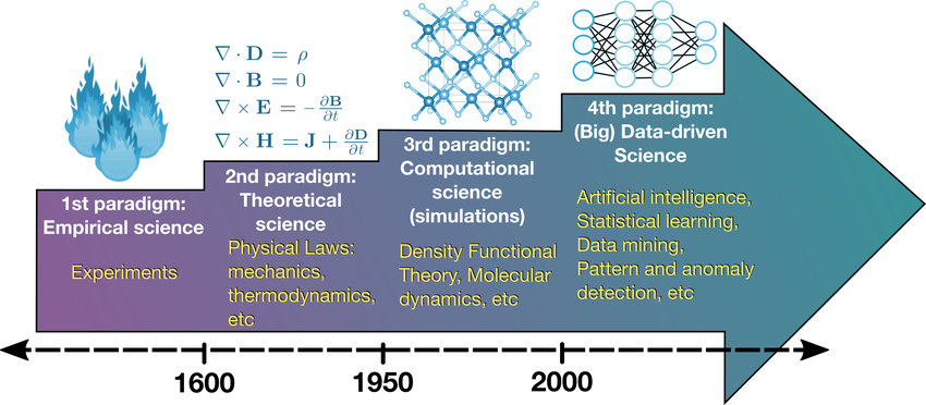
Computer science changed science and engineering forever!
Some commonly used software suites are MATLAB and Octave. However, Python is also VERY powerful with the use of libraries numpy, scipy and matplotlib.
2 NumPy Basics
NumPy aims to provide an array object that is up to 50x faster than traditional Python lists. It is called ndarray.
They also can be multidimensional and have a lot of supporting mathematical operations.
For example, observe some differences:
import numpy as nplist1 = [15.5, 25.11, 19.0]list2 = [12.2, 1.3, 6.38] # Create two 1-dimensional (1D) arrays# with the elements of the above listsarray1 = np.array(list1)array2 = np.array(list2)# Concatenate two listsprint('Concatenation of list1 and list2 =', end=' ')print(list1 + list2)print()# Sum two listsprint('Sum of list1 and list2 =', end=' ')for i inrange(len(list1)):print(list1[i] + list2[i], end=' ') print('\n')# Sum two 1D arraysprint('Sum of array1 and array2 =', end=' ')print(array1 + array2)
Concatenation of list1 and list2 = [15.5, 25.11, 19.0, 12.2, 1.3, 6.38]

Sum of list1 and list2 = 27.7 26.41 25.38

Sum of array1 and array2 = [27.7  26.41 25.38]
2.1 Some array properties
Shape: The shape of an array is a tuple of integers indicating the size of the array along each dimension. For a 1D array, the shape is (n,), for a 2D array, it’s (m, n), and so on.
Data Type (dtype): NumPy arrays are homogeneous, meaning all elements must have the same data type. The dtype attribute specifies the data type of the array elements.
import numpy as nparr = np.array([1, 2, 3])print(arr.dtype)
int64
Dimension (ndim): The number of dimensions of an array is given by the ndim attribute.
import numpy as npimport matplotlib.pyplot as plt# Set seed for reproducibilitynp.random.seed(0)# Generate data from different distributionsdata_uniform = np.random.uniform(0, 1, 1000)data_normal = np.random.normal(0, 1, 1000)data_binomial = np.random.binomial(10, 0.5, 1000)data_poisson = np.random.poisson(3, 1000)data_exponential = np.random.exponential(0.5, 1000)# Plot histograms of the generated dataplt.figure(figsize=(12, 8))plt.hist(data_uniform, bins=30, alpha=0.5, label='Uniform')plt.hist(data_normal, bins=30, alpha=0.5, label='Normal')plt.hist(data_binomial, bins=30, alpha=0.5, label='Binomial')plt.hist(data_poisson, bins=30, alpha=0.5, label='Poisson')plt.hist(data_exponential, bins=30, alpha=0.5, label='Exponential')plt.legend()plt.title('Histograms of Data Generated from Different Distributions')plt.xlabel('Value')plt.ylabel('Frequency')plt.show()
Consider a scenario where you have the following system of equations:
2x + 3y - z = 1
4x + y + 2z = -2
x - 2y + 3z = 3
import numpy as np# Coefficient matrixA = np.array([[2, 3, -1], [4, 1, 2], [1, -2, 3]])# Right-hand side of the equationsB = np.array([1, -2, 3])# Solve the system of equationssolution = np.linalg.solve(A, B)# Print the solutionprint("Solution:")print("x =", solution[0])print("y =", solution[1])print("z =", solution[2])
Solution:
x = -6.000000000000001
y = 6.8571428571428585
z = 7.571428571428572
In this example, we create a 3x3 coefficient matrix A representing the coefficients of x, y, and z in each equation. We also create a 1x3 array B representing the right-hand side of the equations.
We then use np.linalg.solve to solve the system of equations Ax = B for x, y, and z. The solution gives the values of x, y, and z that satisfy all three equations simultaneously.
2.5.5 Example: fitting a polynomial
import numpy as npimport matplotlib.pyplot as plt# Generate some noisy data pointsnp.random.seed(0)x = np.linspace(0, 10, 50)y =2.5* x**3-1.5* x**2+0.5* x + np.random.normal(size=x.size)*50# Fit a polynomial curve to the datacoefficients = np.polyfit(x, y, 3) # Fit a 3rd-degree polynomialpoly = np.poly1d(coefficients)y_fit = poly(x)# Plot the original data and the fitted curveplt.figure(figsize=(10, 6))plt.scatter(x, y, label='Data')plt.plot(x, y_fit, color='red', label='Fit')plt.xlabel('x')plt.ylabel('y')plt.title('Polynomial Curve Fitting')plt.legend()plt.show()
2.5.6 Example: a digital elevation model (DEM)
Given a DEM represented by a 2D NumPy array, the slope at each point can be calculated using the gradient method. The gradient method calculates the rate of change of elevation in the x and y directions, which can be used to determine the slope. This is very useful in many geoscience applications.
import numpy as np# Sample elevation data (DEM)x, y = np.meshgrid(np.linspace(-10, 10, 100), np.linspace(-10, 10, 100))elevation_data = np.sin(np.sqrt(x**2+ y**2))print(elevation_data)# Calculate the gradients in the x and y directionsdx, dy = np.gradient(elevation_data)# Calculate the slope magnitudeslope = np.sqrt(dx**2+ dy**2)print("Slope at each point:")print(slope)
In this example, we first calculate the gradients dx and dy in the x and y directions using np.gradient. Then, we calculate the slope magnitude at each point using the formula slope = sqrt(dx^2 + dy^2).
We can even use matplotlib to visualize the elevation and gradient:
plt.figure(figsize=(10, 8))plt.imshow(elevation_data, cmap='terrain', origin='lower', extent=(-10, 10, -10, 10))plt.colorbar(label='Elevation')plt.title('Digital Elevation Model (DEM)')plt.xlabel('X')plt.ylabel('Y')# Plot the gradient as quiver arrowsskip =4plt.quiver(x[::skip, ::skip], y[::skip, ::skip], dx[::skip, ::skip], dy[::skip, ::skip], scale=5, color='red', alpha=0.7)plt.show()
3 The SciPy Library
Builds on NumPy arrays and matrices and provides lots of functions that perform scientific calculations on them.
See, for example, these submodules:
Integration (scipy.integrate): Provides functions for numerical integration, including single and multiple integrals, as well as solving ordinary differential equations (ODEs).
Optimization (scipy.optimize): Offers optimization algorithms for finding the minimum or maximum of a function, both constrained and unconstrained, and for curve fitting.
Interpolation (scipy.interpolate): Contains functions for interpolating data, including linear, polynomial, and spline interpolation.
Linear Algebra (scipy.linalg): Provides functions for performing linear algebra operations, such as solving linear systems, computing eigenvalues and eigenvectors, and singular value decomposition (SVD).
Statistics (scipy.stats): Contains a wide range of probability distributions and statistical functions for calculating statistics, generating random numbers, and performing hypothesis testing.
Signal Processing (scipy.signal): Offers functions for signal processing, including filtering, spectral analysis, and waveform generation.
Fast Fourier Transform (scipy.fft): Provides functions for computing the discrete Fourier transform (DFT) and its inverse, as well as for working with Fourier transforms in general.
Sparse matrices (scipy.sparse): Contains functions for working with sparse matrices, including creating sparse matrices, performing matrix-vector multiplication, and solving linear systems.
Spatial algorithms (scipy.spatial): Provides functions for working with spatial data structures and algorithms, such as nearest-neighbor queries and Delaunay triangulations.
Image Processing (scipy.ndimage): Offers functions for image processing tasks, such as filtering, morphological operations, and measurements on images.
3.1 Example: integration
\[
y = \int_{0}^{1}(x^2 + 2x) dx
\]
import scipy.integrate as spi# Define the function to be integrateddef f(x):return x**2+2*x# Calculate the definite integral of f(x) from 0 to 1result, error = spi.quad(f, 0, 1)print("Result:", result)print("Error:", error)
3.2 Example: calculating the frequency spectrum of a signal
import numpy as npimport matplotlib.pyplot as pltfrom scipy.fft import fft, fftfreq# Generate a sample signalfs =1000# Sampling frequencyt = np.linspace(0, 1, fs, endpoint=False) # Time vector from 0 to 1 secondf1, f2 =10, 100# Frequencies of the two components of the signalsignal = np.sin(2* np.pi * f1 * t) +0.5* np.sin(2* np.pi * f2 * t) # Signal with two components# Compute the FFTfft_result = fft(signal)magnitude = np.abs(fft_result)frequencies = fftfreq(len(signal), 1/fs)# Plot the signalplt.figure(figsize=(12, 6))plt.subplot(2, 1, 1)plt.plot(t, signal)plt.title('Input Signal')plt.xlabel('Time (s)')plt.ylabel('Amplitude')# Plot the frequency spectrumplt.subplot(2, 1, 2)plt.plot(frequencies[:fs//2], magnitude[:fs//2]) # Plot only the positive frequenciesplt.title('Frequency Spectrum')plt.xlabel('Frequency (Hz)')plt.ylabel('Magnitude')plt.tight_layout()plt.show()
3.3 Exercise: plotting a Voronoi diagram from a random collection of points.